Understanding Vectors in Linear Algebra with Python

5 minute read

Published: February 05, 2023

Understanding Vectors in Linear Algebra with Python

Introduction

Linear algebra is a cornerstone of mathematics, data science, and machine learning. At its core, linear algebra deals with vectors and matrices. Vectors, in particular, are fundamental structures that represent quantities having both magnitude and direction. In this beginner-friendly guide, we’ll explore the concept of vectors, how to perform basic operations on them, and how to use Python (with the NumPy library) to make working with vectors more intuitive and efficient.

What is a Vector?

A vector is an ordered list of numbers. In two dimensions, it can be thought of as an arrow pointing from the origin to a point (x, y). In higher dimensions, vectors are similarly defined, with coordinates in 3D (x, y, z), 4D, or more.

Examples of vectors:

• 2D vector: [3, 4]
• 3D vector: [1, 2, 5]

Vectors have a variety of applications, including:

• Representing spatial points or movements.
• Defining directions in machine learning algorithms.
• Modeling forces in physics.

Mathematical vs. Python Vectors

In mathematics, vectors are typically represented as column vectors or row vectors, with dimensions explicitly indicated. For example, a 3-dimensional column vector might be written as:

[\begin{bmatrix} 1 \ 2 \ 3 \end{bmatrix}]

In Python, vectors are represented using arrays. NumPy, a popular library for numerical computing, uses 1-dimensional arrays for vectors:

import numpy as np
vec = np.array([1, 2, 3])  # Orientationless 1D array.

Python Arrays vs. Mathematical Vectors

1. Dimension Differences: In mathematics, the dimensionality of a vector refers to its number of elements. In Python, a vector is treated as a one-dimensional array (shape (n,)) unless explicitly reshaped into a row (1, n) or column (n, 1) vector.

2. Row vs. Column Representation: Consider the following examples:

asList = [1, 2, 3]         # Python list
asArray = np.array([1, 2, 3])  # 1D array
rowVec = np.array([[1, 2, 3]]) # Row vector (1, 3)
colVec = np.array([[1], [2], [3]]) # Column vector (3, 1)

print(f'asList:  {np.shape(asList)}')
print(f'asArray: {asArray.shape}')
print(f'rowVec:  {rowVec.shape}')
print(f'colVec:  {colVec.shape}')

Output:

asList:  (3,)
asArray: (3,)
rowVec:  (1, 3)
colVec:  (3, 1)

This distinction is important, especially when performing matrix operations, where the orientation (row vs. column) can affect results. Although a 1D array in NumPy looks like a row vector when printed, it does not carry explicit row or column orientation. Understanding this nuance helps prevent errors and aids in debugging.

Creating Vectors in Python

Using Python’s NumPy library makes it easy to create and manipulate vectors. First, install NumPy if you haven’t already:

pip install numpy

Then, import it into your code:

import numpy as np

Let’s create a simple vector:

vector_2d = np.array([3, 4])
vector_3d = np.array([1, 2, 5])

print("2D Vector:", vector_2d)
print("3D Vector:", vector_3d)

Output:

2D Vector: [3 4]
3D Vector: [1 2 5]

Basic Operations on Vectors

1. Vector Addition

When you add two vectors, you add their corresponding components:

vec1 = np.array([1, 2])
vec2 = np.array([3, 4])

result = vec1 + vec2
print("Vector Addition:", result)

Output:

Vector Addition: [4 6]

2. Scalar Multiplication

Multiplying a vector by a scalar (a single number) scales each component:

scalar = 3
vec = np.array([2, 4])

scaled_vec = scalar * vec
print("Scalar Multiplication:", scaled_vec)

Output:

Scalar Multiplication: [ 6 12]

3. Dot Product

The dot product is a fundamental operation in linear algebra, often used to find the angle between vectors or compute projections.

vec1 = np.array([1, 2, 3])
vec2 = np.array([4, 5, 6])

result = np.dot(vec1, vec2)
print("Dot Product:", result)

Output:

Dot Product: 32

Explanation:

(1 * 4) + (2 * 5) + (3 * 6) = 32

Distributive Property of the Dot Product

The dot product satisfies the distributive property:

[A \cdot (B + C) = A \cdot B + A \cdot C]

Example:

A = np.array([1, 2])
B = np.array([3, 4])
C = np.array([5, 6])

left_side = np.dot(A, B + C)
right_side = np.dot(A, B) + np.dot(A, C)

print("Left Side (A dot (B + C)):", left_side)
print("Right Side (A dot B + A dot C):", right_side)

Output:

Left Side (A dot (B + C)): 26
Right Side (A dot B + A dot C): 26

4. Vector Magnitude (Length)

The magnitude (or length) of a vector [x, y] is calculated using the formula:

[\text{magnitude} = \sqrt{x^2 + y^2}]

In Python:

vec = np.array([3, 4])
magnitude = np.linalg.norm(vec)
print("Vector Magnitude:", magnitude)

Output:

Vector Magnitude: 5.0

Vector Applications

1. Unit Vectors: A unit vector has a magnitude of 1 and is used to represent direction. To normalize a vector (convert it to a unit vector):

vec = np.array([3, 4])
unit_vector = vec / np.linalg.norm(vec)
print("Unit Vector:", unit_vector)

Output:

Unit Vector: [0.6 0.8]

1. Projection of a Vector: The projection of vector A onto vector B is given by:

[\text{Projection} = \frac{A \cdot B}{|B|^2} B]

In Python:

A = np.array([3, 4])
B = np.array([1, 2])

projection = (np.dot(A, B) / np.dot(B, B)) * B
print("Projection of A onto B:", projection)

Conclusion

Vectors are a foundational concept in linear algebra and are integral to many areas of data science, machine learning, and physics. With Python and NumPy, you can easily perform vector operations, making complex mathematical computations simple and efficient. Mastering these basics will prepare you for deeper explorations into linear transformations, eigenvalues, and other advanced topics. Happy coding!

Easy NumPy Beginner Guide

6 minute read

Published: February 04, 2023

A Beginner’s Guide to Numpy: Unlocking the Power of Python for Data Science

Introduction

In the world of data science and machine learning, Numpy stands as one of the foundational libraries in Python. Short for Numerical Python, Numpy provides powerful tools to handle large, multi-dimensional arrays and matrices. It also includes a collection of mathematical functions to perform operations on these data structures efficiently. If you’re new to Numpy, this guide will walk you through its basics, giving you a strong foundation for more advanced data analysis tasks.

A Brief History of Numpy

Numpy was created by Travis Oliphant in 2006 by combining the features of two earlier libraries: Numeric and Numarray. The goal was to unify these libraries into a more powerful and comprehensive tool for scientific computing in Python. Over the years, Numpy has grown into one of the most widely used libraries in the Python ecosystem, providing the foundation for more specialized tools like Pandas, Scikit-learn, and TensorFlow. Its open-source nature and active community have driven continuous improvements and optimizations.

Why Use Numpy?

Before diving into how to use Numpy, let’s look at why it’s so popular:

1. Performance: Numpy arrays are more efficient than Python lists, both in terms of memory usage and computation speed.
2. Convenience: It provides an extensive suite of functions for mathematical, statistical, and linear algebra operations.
3. Interoperability: Numpy works seamlessly with other libraries like Pandas, Matplotlib, and Scikit-learn.

Installing Numpy

To start using Numpy, you first need to install it. You can do this using pip:

pip install numpy

Once installed, import it into your Python environment:

import numpy as np

The as np is a common alias that makes the code cleaner and easier to read.

Core Concepts and Basic Operations

1. Creating Numpy Arrays

The fundamental object in Numpy is the ndarray (n-dimensional array). Let’s look at how to create one:

import numpy as np

# Creating a 1D array
arr1 = np.array([1, 2, 3, 4, 5])

# Creating a 2D array
arr2 = np.array([[1, 2, 3], [4, 5, 6]])

print(arr1)
print(arr2)

Output:

[1 2 3 4 5]
[[1 2 3]
 [4 5 6]]

2. Array Attributes

Numpy arrays come with several useful attributes:

print(arr2.shape)  # Output: (2, 3)
print(arr2.ndim)   # Output: 2
print(arr2.size)   # Output: 6

• shape gives the dimensions of the array.
• ndim returns the number of dimensions.
• size shows the total number of elements.

3. Array Operations

Numpy makes element-wise operations simple:

arr = np.array([10, 20, 30])

# Adding a scalar
print(arr + 5)  # Output: [15 25 35]

# Element-wise multiplication
print(arr * 2)  # Output: [20 40 60]

4. Matrix Operations

Matrix manipulation is a core feature of Numpy:

A = np.array([[1, 2], [3, 4]])
B = np.array([[5, 6], [7, 8]])

# Matrix addition
print(A + B)

# Matrix multiplication
print(np.dot(A, B))

5. Dot Product and Distributive Property

The dot product is a key operation in linear algebra, used frequently in machine learning and data analysis:

vec1 = np.array([1, 2, 3])
vec2 = np.array([4, 5, 6])

# Dot product
dot_product = np.dot(vec1, vec2)
print(dot_product)  # Output: 32

Explanation: The dot product of [1, 2, 3] and [4, 5, 6] is computed as:

(1*4) + (2*5) + (3*6) = 32

Numpy also adheres to distributive properties:

A = np.array([1, 2, 3])
B = np.array([4, 5, 6])
C = np.array([7, 8, 9])

# Distributive property
left = np.dot(A, B + C)
right = np.dot(A, B) + np.dot(A, C)

print(left == right)  # Output: True

This shows that A · (B + C) = A · B + A · C, confirming the distributive nature of the dot product.

6. Slicing and Indexing

Accessing specific elements, rows, or columns is straightforward:

arr = np.array([10, 20, 30, 40, 50])
print(arr[1:4])  # Output: [20 30 40]

In a 2D array:

arr2 = np.array([[1, 2, 3], [4, 5, 6]])
print(arr2[1, 2])  # Output: 6
print(arr2[:, 1])  # Output: [2 5]

NumPy Basics: Arrays and Vectorized Computation

One of the core strengths of Numpy is its support for vectorized computation, which allows you to perform operations on entire arrays without using explicit loops. This makes your code more concise and efficient.

1. Vectorized Arithmetic Operations

Numpy allows arithmetic operations to be applied directly to arrays:

arr = np.array([1, 2, 3, 4])

# Vectorized addition
print(arr + 10)  # Output: [11 12 13 14]

# Vectorized multiplication
print(arr * 3)  # Output: [ 3  6  9 12]

These operations are significantly faster than looping through elements using standard Python lists.

2. Element-wise Operations with Two Arrays

arr1 = np.array([1, 2, 3])
arr2 = np.array([4, 5, 6])

# Addition
print(arr1 + arr2)  # Output: [5 7 9]

# Multiplication
print(arr1 * arr2)  # Output: [ 4 10 18]

3. Mathematical Functions

Numpy provides a suite of functions for mathematical computations:

arr = np.array([0, np.pi/2, np.pi])

print(np.sin(arr))  # Output: [0. 1. 0.]
print(np.exp(arr))  # Exponential function
print(np.sqrt(arr)) # Square root (note: sqrt(0) = 0)

Common Numpy Functions

1. Generating Arrays:
   • np.zeros((3, 3)) – Creates a 3x3 array of zeros.
   • np.ones((2, 4)) – Creates a 2x4 array of ones.
   • np.linspace(0, 10, 5) – Generates five equally spaced values between 0 and 10.
2. Statistical Functions:
   • np.mean(arr) – Computes the mean.
   • np.std(arr) – Computes the standard deviation.
   • np.sum(arr) – Computes the sum of array elements.
3. Random Numbers:
   • np.random.rand(3, 3) – Generates a 3x3 matrix with random numbers between 0 and 1.
   • np.random.randint(1, 100, size=(2, 3)) – Generates a 2x3 matrix of random integers between 1 and 99.

Conclusion

Numpy is a powerful and indispensable tool for anyone working with numerical data in Python. Mastering its core features will help you build efficient, scalable solutions for data analysis, machine learning, and beyond. Vectorized computation is one of its key strengths, making complex calculations straightforward and efficient. As you advance, you’ll discover even more sophisticated operations that can be performed with Numpy. Happy coding!

Feature Engineering Explained

4 minute read

Published: February 03, 2023

Feature Engineering: Unlocking the Power of Data for Machine Learning

Linear Regression Simply Explained

6 minute read

Published: February 01, 2023

Linear Regression Explained

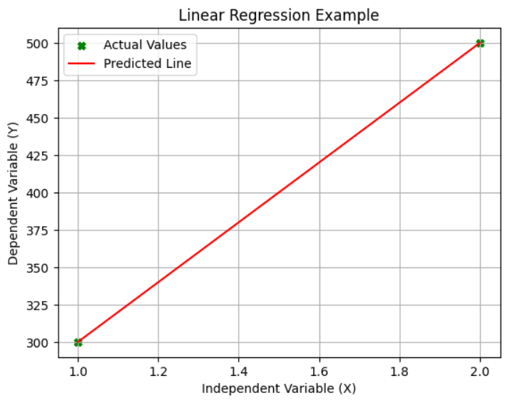
Linear regression is a statistical method used to model and understand the relationship between variables:

• One or more independent variables (X)
• One dependent variable (Y)

Linear regression finds a line that best fits the dataset. This line helps predict the dependent variable (Y) based on the independent variable(s) (X).

Use Cases

1. Predicting House Prices
2. Stock Price Prediction
3. Medical Cost Estimation
4. Sales Forecasting

Key Points

• Y: the values you want to predict
• X: the values used to make the prediction

Mathematical Interpretation

For simple linear regression (with one independent variable), the equation is:

Y = wX + b

Where:

• w (weight or slope) represents the change in Y for each unit change in X.
• X is the independent variable.
• b (bias or intercept) is the value of Y when X is 0.

In more complex cases with multiple independent variables, this equation can be extended to:

Y = w1X1 + w2X2 + ... + wnXn + b

This is called multiple linear regression.

Basic Example

Let’s start with a simple example of linear regression using a dataset with one independent variable (X) and one dependent variable (Y).

Code Implementation

import numpy as np
import matplotlib.pyplot as plt

# Define the dataset
X = np.array([1, 2])  # Independent variable
Y = np.array([300, 500])  # Dependent variable (target values)

# Choose arbitrary values for weight (w) and bias (b)
w = 200  # Weight
b = 100  # Bias

# Calculate predicted Y values using the linear equation Y = wX + b
predicted_Y = w * X + b

# Print predicted values for clarity
for i in range(len(X)):
    print(f"Predicted Y for X={X[i]}: {predicted_Y[i]}")

Explanation

In this example, we are manually defining the weight ((w)) and bias ((b)) of the linear equation:

[ Y = wX + b ]

Predictions

Using the given values for (w) and (b), we can compute the predicted values of (Y):

• For (X = 1): [ Y = (200 \times 1) + 100 = 300 ]
• For (X = 2): [ Y = (200 \times 2) + 100 = 500 ]

These calculations yield the predicted values of (Y) that perfectly match our actual values in the dataset.

Important Note

This example is very basic and uses arbitrary values for (w) and (b) to illustrate the concept of linear regression. In real-world applications, we typically use a cost function (like mean squared error) to optimize these parameters based on the data, allowing the model to learn the best-fit line automatically.

Visualization

To visualize how well our predicted values align with the actual data points, we can create a scatter plot and draw the regression line:

# Visualization
plt.scatter(X, Y, marker="X", c="g", label="Actual Values")
plt.plot(X, predicted_Y, label="Predicted Line", color='r')
plt.title('Linear Regression Example')
plt.xlabel('Independent Variable (X)')
plt.ylabel('Dependent Variable (Y)')
plt.legend()
plt.grid()
plt.show()

Interpretation of the Visualization

In the visualization:

• Green Markers (Actual Values): These represent the actual data points in our dataset.
• Red Line (Predicted Line): This line represents our model’s predictions based on the chosen (w) and (b). It shows how well the model fits the actual data.

scikit-learn implementation

from sklearn.linear_model import LinearRegression
import numpy as np
import matplotlib.pyplot as plt

# Data
X = np.array([[1], [2]])  # Features should be 2D for sklearn
Y = np.array([300, 500])  # Target values

# Linear regression model
model = LinearRegression()
model.fit(X, Y)

# Predict values
predicted_Y = model.predict(X)

# Plotting
plt.scatter(X, Y, marker="X", c="g", label="Actual Value")
plt.plot(X, predicted_Y, label="Our prediction")
plt.legend()
plt.show()

Implementing Linear Regression from Scratch

Let’s implement simple linear regression from scratch using Python:

The Cost Function

To assess how well our model fits the data, we use the Mean Squared Error (MSE) cost function:

[MSE = \frac{1}{n} \sum_{i=1}^{n} (y_{i} - \hat{y}_{i})^2]

Where:

• \(n\) is the number of samples.
• \(y_{i}\) is the actual value.
• \(\hat{y}_{i}\) is the predicted value.

Gradient Descent

To optimize our model, we employ the gradient descent algorithm, which minimizes the cost function by iteratively adjusting the weights and bias. The update rules for the weights and bias are given by:

[\beta_j = \beta_j - \alpha \cdot \frac{\partial MSE}{\partial \beta_j}]

Where:

• \(\beta_j\) represents the weights (or bias).
• \(\alpha\) is the learning rate, controlling the size of the steps taken towards the minimum.

Code Implementation

Let’s dive into the code for our Linear Regression model.

import numpy as np

class LinearRegression():
    def __init__(self, learning_rate, max_iter):
        self.lr = learning_rate
        self.max_iter = max_iter

    def fit(self, X, y):
        n_samples, n_features = X.shape
        
        self.weights = np.random.rand(n_features)
        self.bias = 0

        for _ in range(self.max_iter):
            y_pred = np.dot(X, self.weights) + self.bias
            dw = (1 / n_samples) * np.dot(X.T, (y_pred - y))
            db = (1 / n_samples) * np.sum(y_pred - y)

            self.weights -= self.lr * dw
            self.bias -= self.lr * db

    def predict(self, X):
        return np.dot(X, self.weights) + self.bias
    

if __name__ == "__main__":
    from sklearn.datasets import make_regression
    from sklearn.model_selection import train_test_split
    from sklearn.metrics import mean_squared_error

    X, y = make_regression(n_samples=200, n_features=1, noise=10, random_state=42)

    X_train, X_test, y_train, y_test = train_test_split(X, y, test_size=0.2, random_state=42)
    reg = LinearRegression(learning_rate=0.01, max_iter=1000)
    reg.fit(X=X_train, y=y_train)
    y_pred = reg.predict(X_test)

    print(f"{mean_squared_error(y_test, y_pred):.3f}")

This implementation uses gradient descent to minimize the mean squared error and find the optimal weights and bias.

Using Scikit-learn for Linear Regression

Now, let’s implement the same linear regression using scikit-learn:

from sklearn.datasets import make_regression
from sklearn.model_selection import train_test_split
from sklearn.metrics import mean_squared_error
import matplotlib.pyplot as plt
from sklearn.linear_model import LinearRegression

X, y = make_regression(n_samples=200, n_features=1, noise=10, random_state=42)

X_train, X_test, y_train, y_test = train_test_split(X, y, test_size=0.2, random_state=42)

model = LinearRegression()
model.fit(X_train, y_train)

y_pred = model.predict(X_test)

print(mean_squared_error(y_test, y_pred))

plt.scatter(X_test, y_test, color='blue')
plt.plot(X_test, y_pred)
plt.xlabel('X')
plt.ylabel('y')
plt.title('Linear Regression Dataset')
plt.show()

This scikit-learn implementation provides a more streamlined approach with built-in features like train-test splitting and model evaluation metrics.

Both implementations demonstrate how to create a linear regression model, fit it to data, make predictions, and visualize the results. The scikit-learn version offers additional functionality and is generally more efficient for real-world applications.

Conclusion

Linear regression is a powerful and widely-used technique in statistics and machine learning. Its simplicity and interpretability make it an excellent starting point for predictive modeling and data analysis. While it has limitations, particularly with complex, non-linear relationships, it remains a fundamental tool in a data scientist’s toolkit.

By understanding the concepts behind linear regression and how to implement it, you’re well on your way to more advanced machine learning techniques. Remember, the key to mastering linear regression is practice – try applying it to various datasets and real-world problems to gain a deeper understanding of its capabilities and limitations.

As you continue your journey in data science and machine learning, you’ll find that the principles you’ve learned here form the foundation for many more advanced techniques. Keep exploring, and happy modeling!